Wetland Feature Maps
Published:
Background
In my PhD, I did a lot of wetland mapping with the Wetland Intrinsic Potential (WIP) tool. This tool was a pixel-based approach meaning that every pixel was modeled using points that extracted feature information at that location. For example a digital elevation model (DEM) would be used to calculate slope and then a point location would extract that slope value for that pixel (or groups of pixels with some sampling interpolation). With a bunch of features, especially those calculated at different length scales See the paper here for details, we could confidently map wetlands using a random forest algorithm and produce a continuous probability.
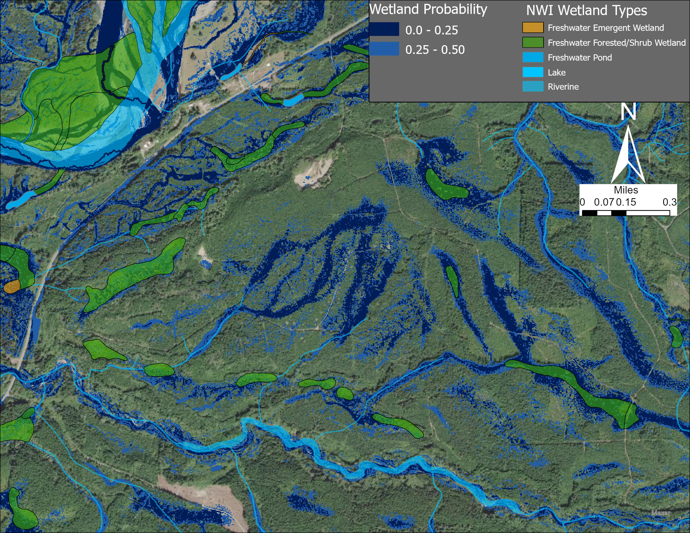
But one thing that these pixel based approaches find difficult is segmenting pixels into objects. In wetland terms, a group of high wetland probability pixels could be grouped into one “wetland”. There are pros/cons to this. Wetlands rarely have sharp boundaries, but often wetland delineations need to establish boundaries for regulations. Segmentation also known as object-based image analysis, can happen before the modeling such as segmenting groups of pixels and then taking a mean of the pixel feature values or other metric to be fed into the model. It can also happen after, which in the WIPs case we could smooth pixel values to remove spotty-ness and gaps and then create groups above certain thresholds.
However, deep learning algorithms are able to complete image segmentation without these pre/post processing steps. These algorithms like convolutional neural networks search images for features then group pixels together based on those features giving each pixel a label and a probability. For wetland mapping this was very interesting since we could tackle the problem of the segmentation with the algorithm.
But what are these deep learning features? In the WIP random forest model, we calculated several of our own features at multiple length scales to capture the spatial variability that might correspond to wetland presence. In convolutional neural networks such as the U-Net, features are captured with convolutions and resampling down to multiple levels of resolution. The features are similar to hot-spots of variation in an image but corresponding to all bands. They might not look anything like the engineered features from terrain that we calculated from WIP.
So that brings me to this attempt to visualize those features as they are built in the deep learning model.
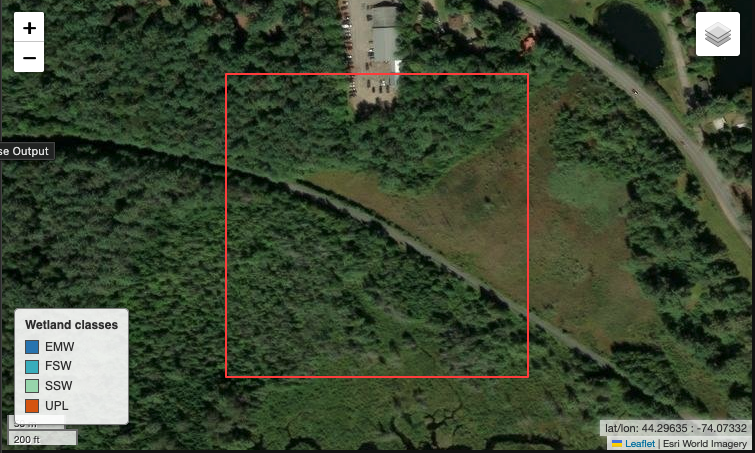
The input data
We’ll use a 256m x 256m image at a 1m resolution so that each pixel is 1mx1m. The image is a stack that contains multiple bands of information to train on for predicting wetland classes. In total there are 19 predictors in these groupings:
| Category | Description |
|---|---|
| Elevation/Terrain | Digital elevation model and terrain derivatives |
| Hydrology | Terrain derived hydrology metrics |
| Imagery | leaf-on and leaf-off imagery |
| Lidar | Percent returns above and below certain thresholds |
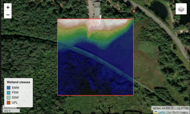
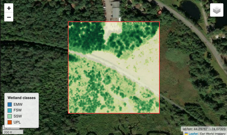
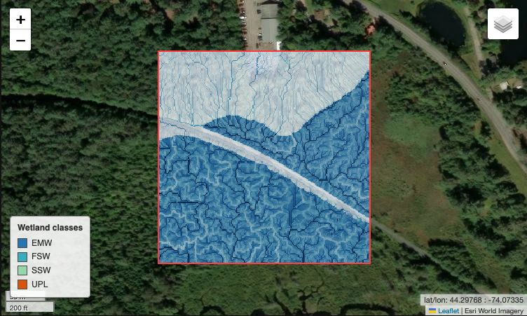
Here are some images of what the patch looks like with some of those bands
The deep learning model architecture
We are using a convolutional neural network architecture called U-Net originally used for medical images it has been adapted to other areas including geospatial. Specifically, we are using U-Net3+ which aims to take advantage of all scales used in the regular U-Net with full-scale skip connections.
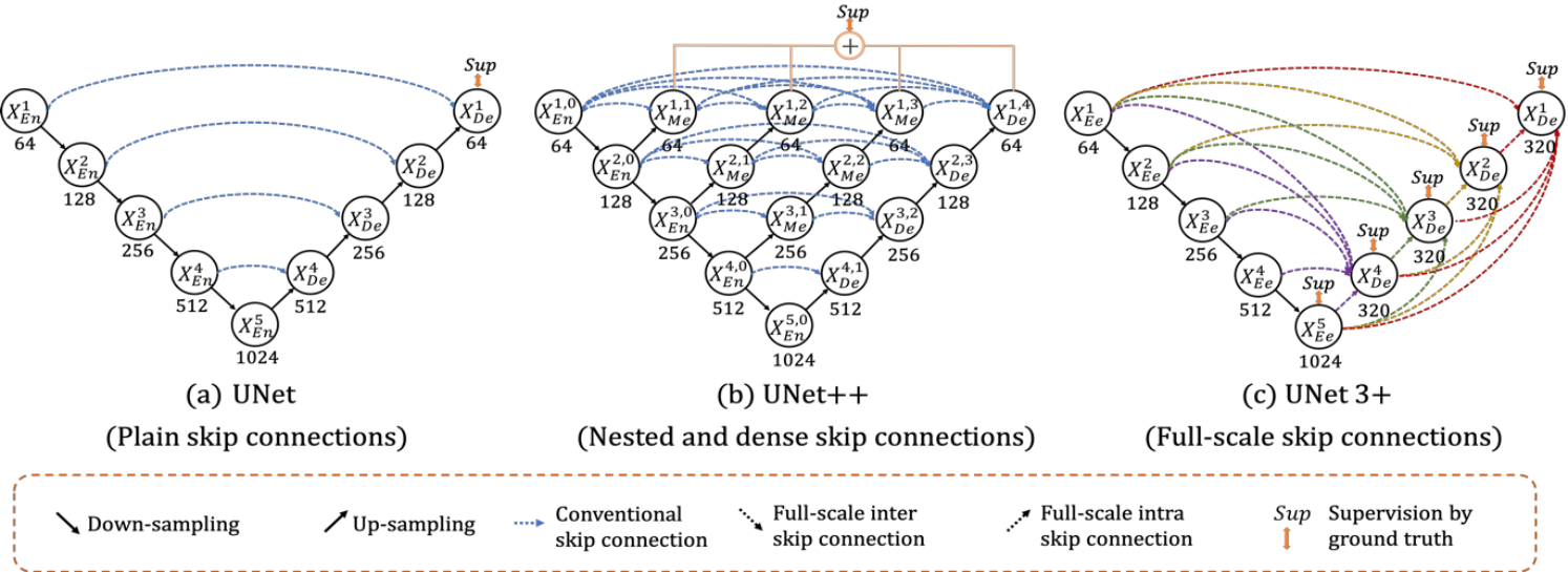
The U-Net architecture has three main components: Encoders, Decoders, and a Bottleneck. Input images (with 19 input bands) from a training dataset enter the model pipeline at the first encoder block. Encoder blocks are where convolution filters are applied and the feature maps are created. The convolution filters are usually 3x3 kernels with weights that are initialized and trained to detect features and use padding to preserve the native resolution (256x256).
In our U-Net the first encoder block uses 64 filters creating 64 feature maps. Feature maps are the models’ representation of the patterns in the input image based on a convolution filter pass. Similar to a user-calculated layer like slope or TWI, the model is using convolution filters to calculate its own features except the values of the convolution are learned during the model training process and the features are a combination of all the predictor bands. Now there are 64 of these!
- Side note: to me,
kernels = filters = moving windowsbut that might be oversimplifying things, since technically the convolution filter works across all the input channels.
With those 64 feature maps, a ReLU (Rectified Linear Unit, outputs 0 for negatives, passes positives unchanged) activation is used to zero out the negative values, introducing non-linearity. Then, a 2x2 kernel for max pooling is used to down-sample the resolution of each of the 64 feature maps (e.g. 256x256 to 128x128). The next encoder doubles the depth of the convolution filters to 128 and then producing 128 feature maps, which similarly go through ReLU activation and max pooling. At each subsequent encoder block, the resolution decreases and feature maps increase in number until it reaches the bottleneck where the lowest resolution but highest number of feature maps reside.
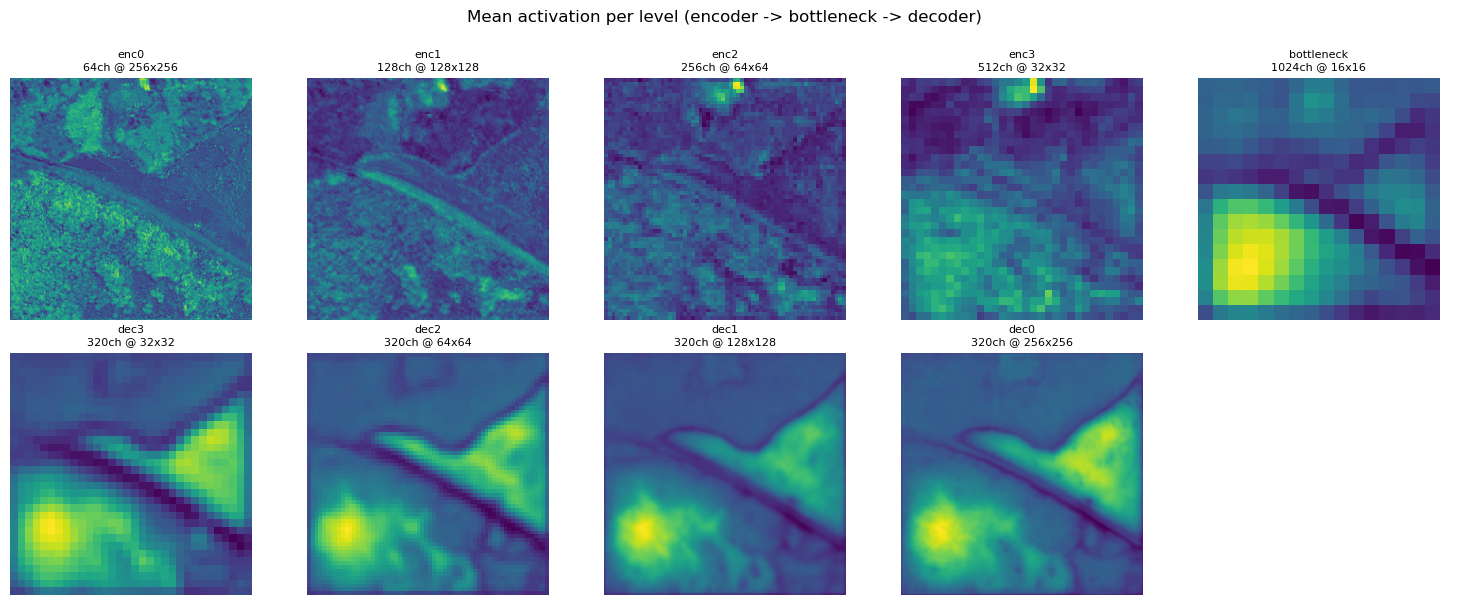
Into the encoders
So once we put our 256m x 256m input image with 19 bands shown above into the encoder, the convolution filters and ReLU start to create feature maps starting with 64 at the first encoder block and doubling at the next. There are tons of these feature maps, for a 4 level depth U-Net that would be 64+128+256+512 = 960 total just from the encoders! Because that’s so many, I’ve taken the highest variance feature maps and show them below.
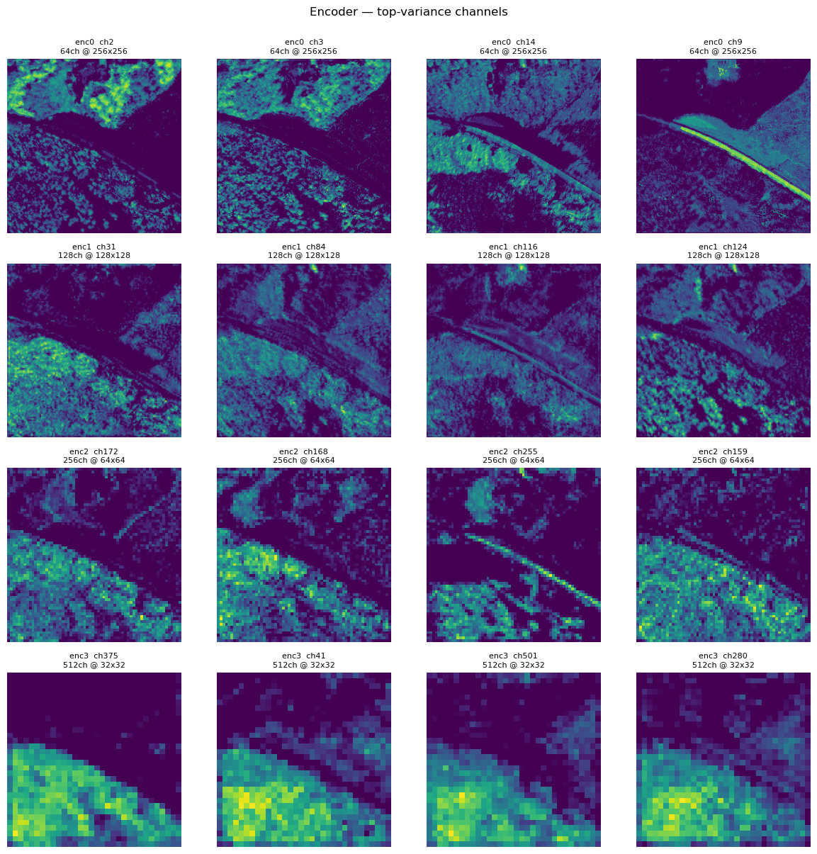
First thing I notice as we get down the encoders the resolution gets coarser. But at the same time, the features go from seemingly random patterns to more recognizable ones from the first image. The road definitely sticks out and same with the forest patch below.
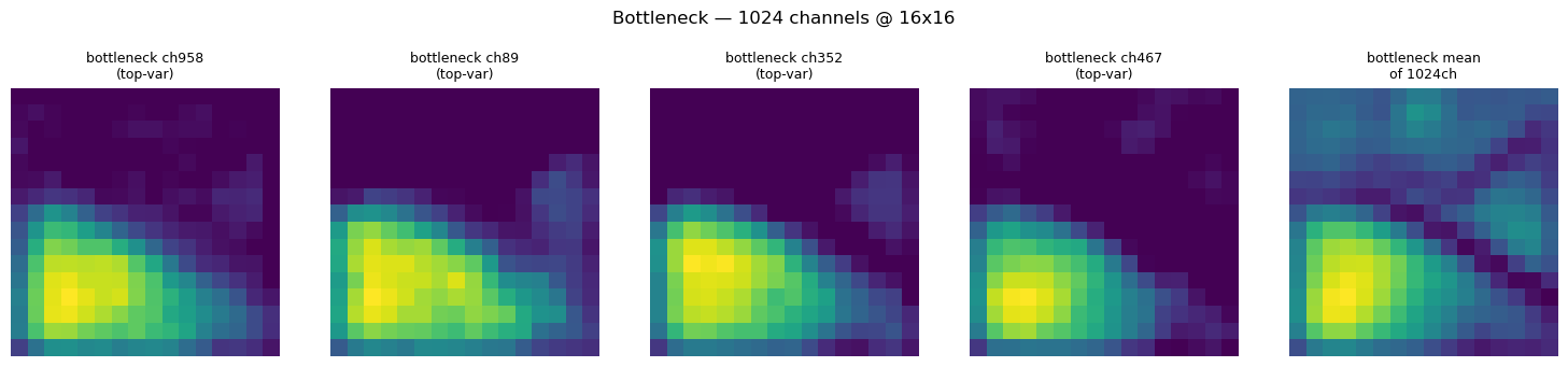
Into the bottlneck
At the bottleneck we see the coarsest resolution feature maps and those patterns from late in the encoder stage are really highlighted. Again this is only a sample of the bottleneck images except for the last image which is a mean of all the channels (1024!). You can definitely see the road and forest stick out and there seems to be some light hot spots in the middle-right and middle-top
Out of the bottleneck and into the decoders
Now the decoders take what was in the bottleneck and start the upsampling process, going from coarse resolution to fine resolution using up-sampling 2x2 convolutions that halve the number of feature channels. But instead of just upsampling, the decoder also concatenates features from the same resolution encoder levels. In the original U-Net these were simple skip connections that worked across one level of encoder-decoder, in the U-Net diagram above on the left. The concatenation works because each encoder block has a corresponding decoder block at the same resolution. So in a four level U-Net the first encoder block concatenates with the fourth (last) decoder block, second encoder to the third decoder, third encoder to the second decoder, and fourth encoder to the first decoder. After each concatenation two 3x3 convolution filters would occur to detect features followed by a ReLU to determine the feature map. The reason for the concatenating is that downsampling loses a lot of spatial detail so the concatenating recovers encoder level detail at the corresponding decoder level.
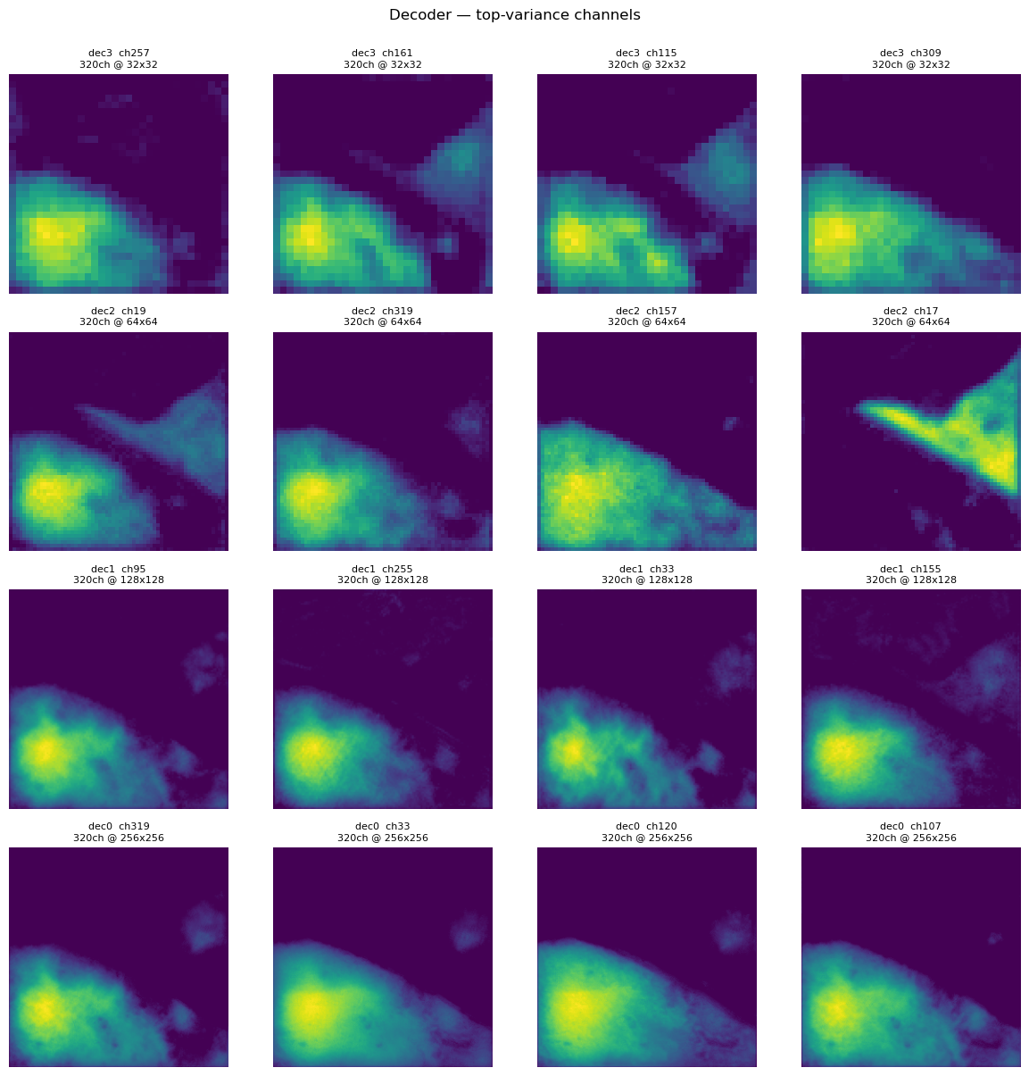
But in U-Net3+ the information from each encoder is shared to each decoder through resampling to a shared resolution and then unified to a set number of channels. The shared number of channels is determined by 64 3x3 convolution filters producing a 64 channel feature map. At each decoder block, aggregating five scales at 64 channels each gives 64×5 = 320. Each decoder then applies further 3x3 convolution filters (320) and batch normalization plus ReLU activation to fuse them.
Another addition to the U-Net3+ model vs. the previous U-Net is the use of deep supervision. This is where the model learns hierarchical representations from the aggregated feature maps produced at each decoder. Essentially the aggregated feature maps at each decoder level produce a prediction via a 3x3 convolution filter, bilinear upsampling to the native resolution, and a softmax activation function. In regular U-Net loss was calculated on the final output at the last decoder layer compared to the ground-truth labels. But with deep supervision each decoder’s prediction gets its own loss, so the correction signal reaches the deeper layers directly rather than only propagating back from the final output. This helps the model learn weights and parameters better than the original U-Net since the signal is not just from the final output at the last decoder which can get lost further into the model.
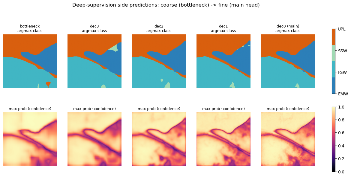
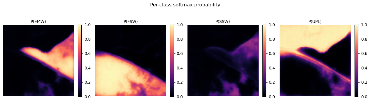
At the final decoder level a final 1x1 convolution condenses the channels down to N-number of channels, one for each class in the classification at the native resolution. The values for each pixel are called a logit and softmax function then converts these logits into 0-1 probabilities. The top probability value, via argmax corresponds to the final predicted class.
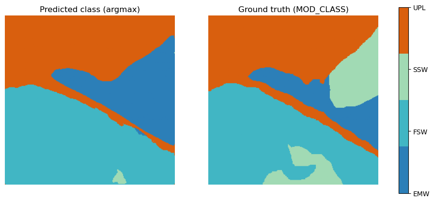
With our example patch there are a couple things to note on how the model worked.
- Generally it got the major patterns right.
- The boundaries of the wetlands overall look about the same as the ground-truth. It especially noticed the road was not part of the wetland complex which makes sense from the previous feature maps.
- It missed the scrub shrub wetland (SSW)
- This was interesting because in the RGB imagery there were some vegetation patterns that appear “shrub-like” but just because we can see it does not mean the model saw enough of these features to classify it correctly. But it did find a higher probability of SSW in places where it was labeled.
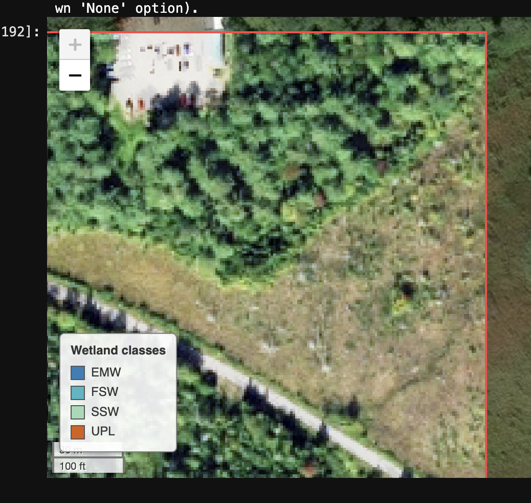
Zooming in on the shrub area
This model was trained pretty lightly on input data compared to most deep learning models. So hopefully we can expect it to improve with more observations. At the same time, there are a lot of deep learning architectures and strategies that can be implemented in these models. A few of them I didn’t mention and am still learning about: loss functions/hybrid loss functions, dual-branch architecture, and attention mechanisms.